
Why this matters? the universal approximation theorem is often misused as a blanket justification for model capability — but understanding what it actually guarantees (and what it doesn’t) reshapes how we think about scaling, memorization, architecture design, and the limits of deep learning.
Assumes familiarity with feed-forward neural nets, activation functions, and the concept of function approximation
Approximation by Superpositions of a Sigmoidal Function by G. Cybenko
We have a representation of a n-dimensional function by linear combination of the form . It basically is a linear combination of sigmoidal outputs of a matrix multiplication of y’s transpose and x plus the corresponding bias. The theorem uses a single hidden layer network and must be non-constant, bounded, continuous, sigmoidal. The is defined as
.
The above constraints are key because they enable us to combine 2 neuron outputs into an if/else statement such as <certain_value> == <threshold> ? 1 : 0 ternary statement. It basically is a table lookup for one variable as follows:
- Neuron 1 emits a step function (a good enough approximation) around a point x, where any value smaller than x results with 0, any value larger or equal to results with 1.
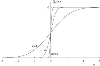
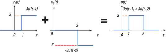
- Neuron 2 emits the same step function with a small shift to the right .
- What we end up with is, 0 for any value < , 1 for any value in , and 2 for any value ≥ , if you combine the outputs of the neurons by adding them (with a weigth 1 each). If you combine them with a weight -1 for the second neuron, you will end up with a 1 for any value in between and , 0 otherwise. Any value larger than , will cause neuron 2 to cancel out neuron 1’s activation. We effectively used 2 neurons to encode one point of the function into the neural network.
If you can find the appropriate combinations of values, you can create a lookup table which gives you 1 for values in it, 0 otherwise. A ‘hash’ set with a neural network… It also gets apparent now that non-linearities are drivers for the lookup table formations in this fashion.
The paper demonstrates that:
“… finite linear combinations of compositions of a fixed, univariate function and a set of affine functionals can uniformly approximate any continuous function of n real variables with support in the unit hypercube; only mild conditions are imposed on the univariate function…”
Meaning that, you can approximate any continuous function which has a non-zero value only in in each of it’s dimensions continuously (support in the unit hypercube) with linear combinations of fixed (continuous function in a range ) and univariate functions (single variable functions within the neuron ) and their affine functions (functions to translate them e.g. shifting the result from 0 to 4).
It does not show how to approximate or how to choose an architecture for the neural network. It just shows that representationally (capacity-wise, there exists at least one neural network that can approximate the function) a neural network can match any function.
We however are interested on learning (compressing) the patterns at hand, not just being able to match a subset of it. It is compression in the sense that it won’t need to ‘memorize’ all the instances and their results, it can ‘reproduce’ them if it extracts the underlying function. Thus, the size of the network should be proportional to the underlying function’s complexity, not the dataset at hand. At a certain point, a sufficiently large neural network should not need to increase in size for it to continue improving (i.e., to avoid increasing validation loss) as the dataset gets larger. If it managed to capture the underlying function, it should not lose performance.
Multilayer Feedforward Networks are Universal Approximators by Kurt Hornik, Maxwell Stinchcombe and Halbert White
‘We have thus established that such “mapping” networks are universal approximators. This implies that any lack of success in applications must arise from inadequate learning, insufficient numbers of hidden units or the lack of a deterministic relationship between input and target.’
It is crucial to note that the deeper neural networks get, the more they can ‘extract’ complexities. A classic example for this is a 3 layer neural network. The first layer finds relevant ‘lines’/’hyperplanes’ i.e. identifies dichotomies learns ‘yes’ or ‘no’s. The next layer combines them by AND or OR to form more complex shapes defining subsets. The last layer includes/excludes those shapes to represent any higher complexity shape.
It seems we don’t still know how deep we should go. More on that later.
If we can say that, any unsuccessful attempt to train a neural network fails because eiher
- inadequate learning
- insufficient numbers of hidden units (does also touch on lookup table size)
- deterministic relationship
is missing, how do we know which one(s)? I am particularly interested in ‘inadequate learning’ which seems to mean the training process cannot find ‘good’ parameters. Since we don’t know how to find the theoretical successful neural networks, or even if there is a way to find them to begin with, it may well mean the case is unlearnable. Or do we even know that the existing ‘solutions’ for the problem are compressed or just lookup tables.
A simple experiment
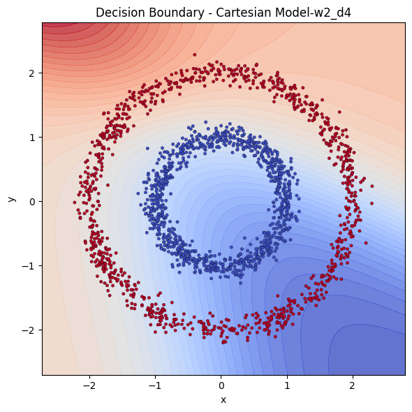
To have a firmer grasp on the above discussion, let us have a toy experiment with single hidden layer networks. This is a widely known example, so you might have seen it before. Imagine having 2 circles, a small and a big one, where the small circle sits in the middle of the big one. We then generate points around the circles with some noise. We want a simple model to learn distinguishing those 2 classes.
You can run this yourself on Google Collab
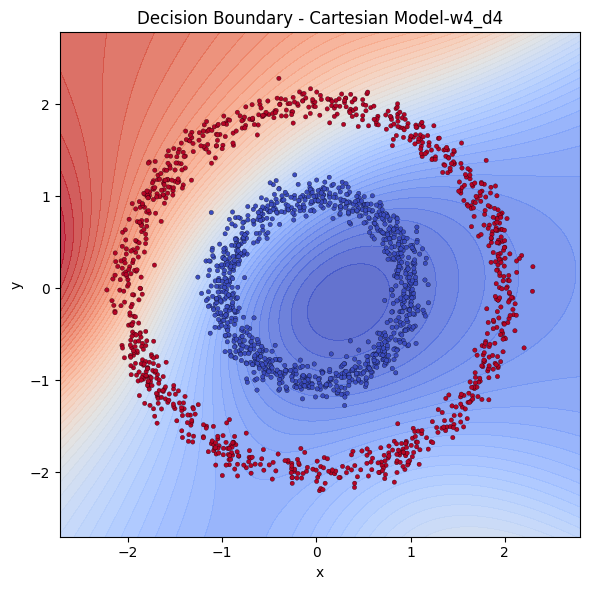
It is immediately visible how we feed the inputs affect the performance. The coordinates can be denoted in Cartesian or Radial coordinates. We see that providing the points in radial coordinates conditions the model by providing the radial structure implicitly. Models that are fed with cartesian coordinates instead seem to struggle to learn. The model does not have to learn that or translate Cartesian to Radial in that case. We have 5 single hidden layered neural networks, 3 cartesian with 4,8 and 64 neurons and 2 radial 4 and 8 neurons. Let’s examine the decision boundaries of those models to see their extraction power.
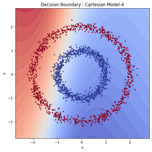
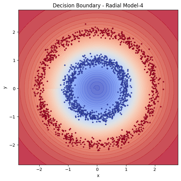
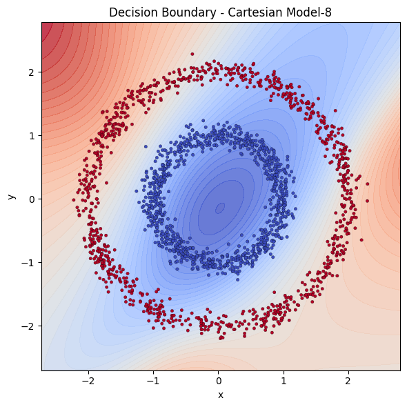
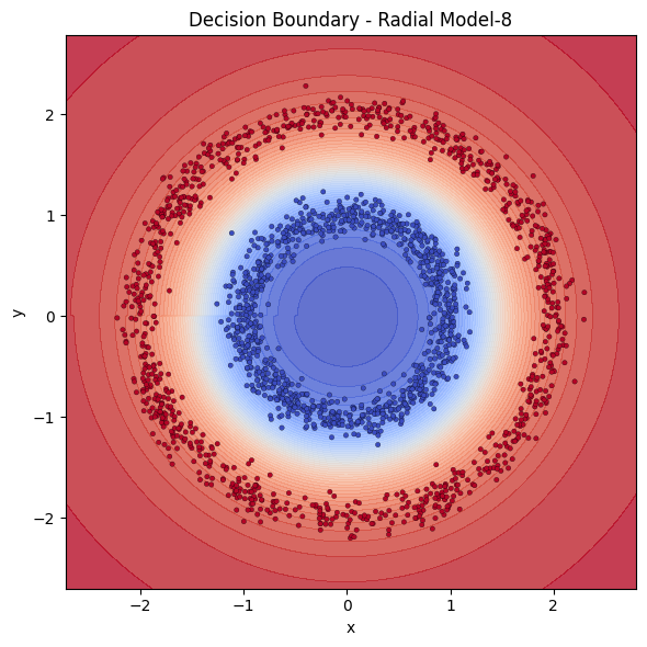
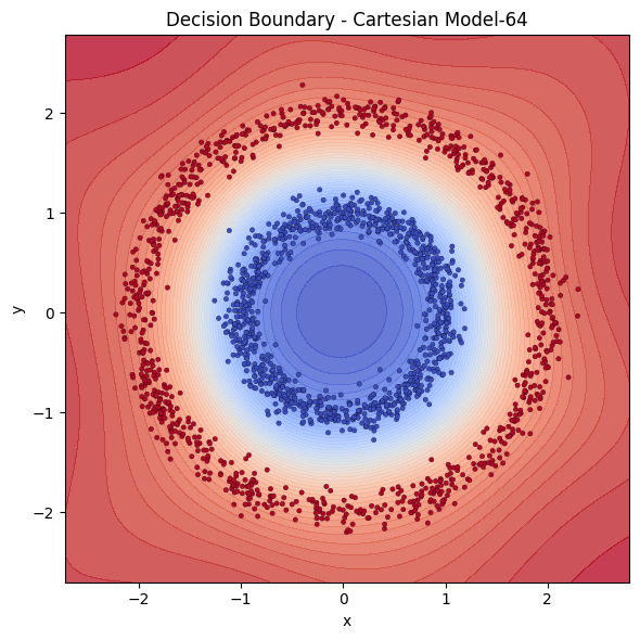
With same power, Cartesian models are destroyed by Radial ones. To catch up with Radial models, Cartesian model needed the square of it’s neurons.
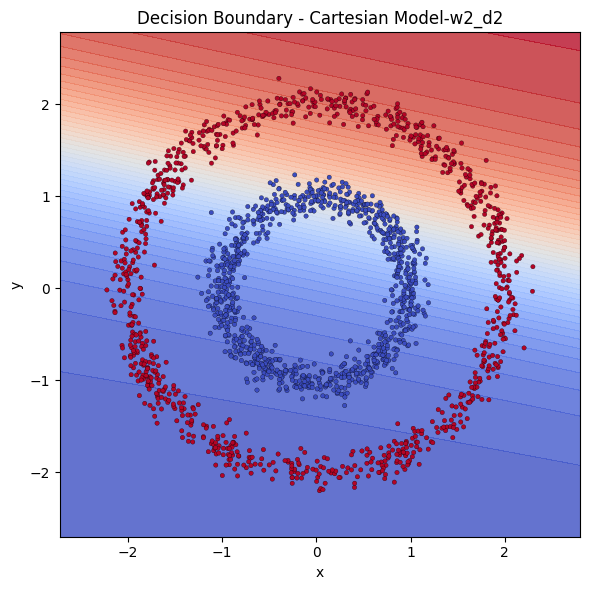
Let’s also test if getting deeper would solve some part of the problem.
Let me show you how their losses to compare them better.
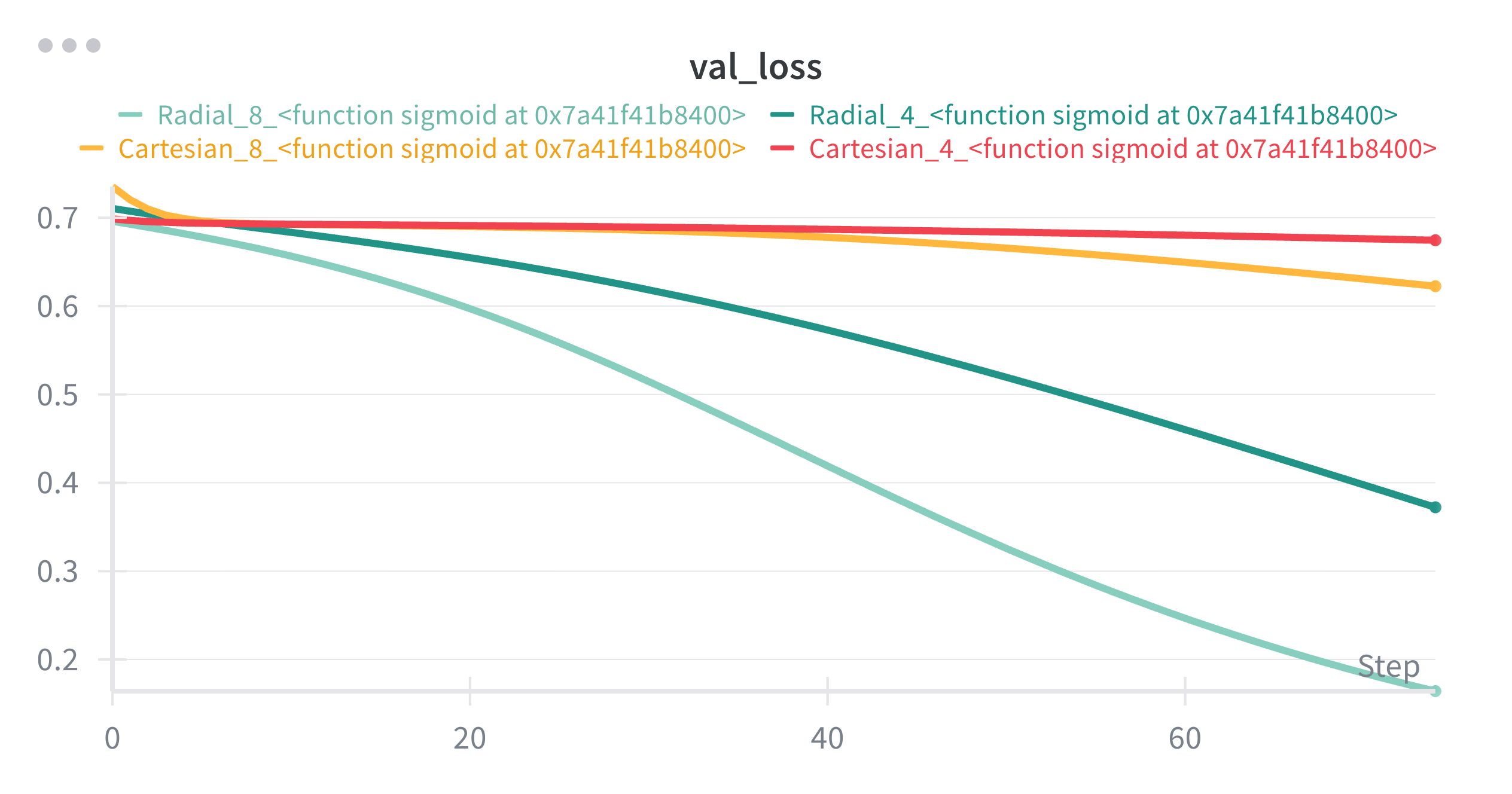
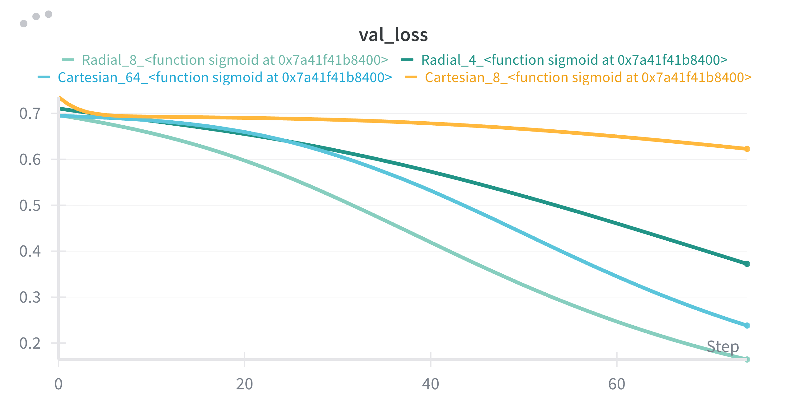
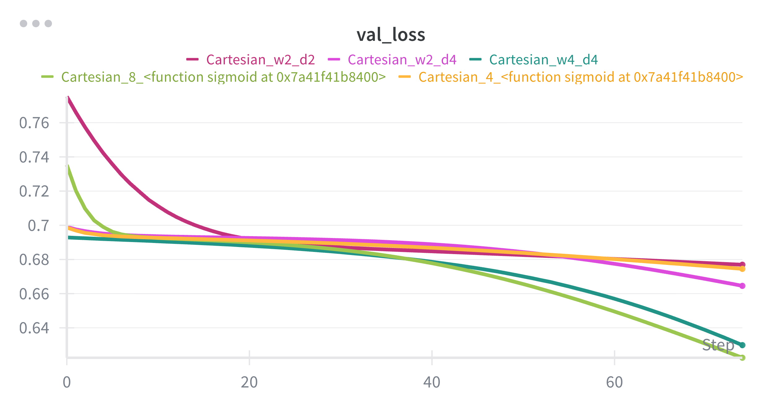
We see that, depth didn’t benefit much, the model 2 hidden layers with 4 neurons each is outperformed by the one a single hidden layer with 8 neurons. Even they both are Cartesian, the wideness seem to benefit more.
I think we can see here that even if the model is not getting best possible input in terms of format, with the enough width, it can learn the underlying function. In our case, with the help of non-linearities, it seems with 64 neurons, our model seems to be able to draw a circle boundary good enough to distinguish 2 classes.
❗ A small implication/take away: if you’re limited in depth or optimizing for simplicity, consider increasing width first—but test depth too because domain matters.
Compression metric T/P : tokens trained on / total number of model parameters
I want to ponder on how ‘good’ the current models compress. Let’s basically compute the ratio between the set of the training set to the parameter count of the model as a metric. Note that this is my ‘proxy’ metric, not something well established in the literature. The data set size is mostly available in terms of tokens. Assuming all the parameter counts include embedding dimensionality as well, if this number goes up, we expect to have compressed more.
| Model | Params (B) | Train. tokens | MMLU (%) | Tokens/Param | Source |
|---|---|---|---|---|---|
| GPT-3 | 175 | 300B | ~43 | 1.71× | (source) |
| Gopher | 280 | 300B | - | 1.07× | (source) |
| Chinchilla | 70 | 1.4T | - | 20.0× | (source) |
| PaLM | 540 | 780B | ~50-53 | 1.44× | (source) |
| Llama 2 (7B) | 7 | 525B | - | 75× | (source) |
| Llama 2 (13B) | 13 | 525B | - | 40.38× | (source) |
| Llama 2 (70B) | 70 | 525B | ~68-71 | 7.5× | (source) |
| Llama 3 (8B) | 8 | 15T (reported) | ~64 | 1875× | (source) |
| Llama 3 (70B) | 70 | 15T (reported) | ~79 | 214.3× | (source) |
| Falcon 40B | 40 | 1.0T | - | 25.0× | (source) |
| MPT-7B | 7 | 1.0T | ~45 (pre-t) | 142.9× | (source) |
| BLOOM 176B | 176 | 350B (logged) | - | 1.99× | (source) |
- MMLU is a benchmark of general knowledge reasoning for Language Models
★ Note on Llama 3: The 15T figure is reported by Meta/Hugging Face blog posts and other summaries; Meta’s technical report/model card with an explicit token count wasn’t published alongside the initial release. Treat these as officially stated via blogs, not a peer-reviewed paper figure
It obviously is another debate if those benchmarks do a good job assessing the performance of the LLM. Furthermore, there were reports showing contamination of test sets or benchmarks. I even think the discrete measurement of performance is not the way to go (MMLU is multiple-choice), (they even caused the ‘emergency’ fallacy).
Observation 1: It is obvious that higher token per parameter ratio does not mean better performance. T/P radically increases for smaller models like LLaMA-2 7B and 13B, but their performance gets worse as parameters decrease — even though “compression pressure” is highest (more data competing for limited weights). We see that large models don’t need high T/P to perform well, PaLM 540B trains at only 1.4× tokens per parameter (low T/P) but greatly outperforms smaller models with vastly higher T/P.
My claim is that additional parameters do improve performance, but not because they’re compressing more of the dataset — they’re allocating capacity to internalizing patterns. One can claim that it is because the capacity (representative or whatever) of smaller models are not enough. I claim otherwise. It just makes more sense to me that bigger models just memorize better than smaller models for the following reasons:
-
Too many tokens per parameter forces abstraction and discourages memorization: Smaller models seeing much higher diversity compared to their parameter count i.e. higher T/P, are discouraged from memorization. It has to perform well on all of them and given it’s small size, it does not have enough room to memorize all of them. Since it cannot extract the underlying functions i.e. compress or learn, it is limited by its size. Larger models do not have that problem because, they have more room to memorize, like they have some room for extra lookup table. I would argue the training process incentivises them to memorize the ones with higher impact first. Thus the diminishing returns of getting large, the outlier memorizations may not even be tested.
-
I think it is reasonable to at least accept that some portion of the sheer volume of giant models are wasted with memorization. Models reproduce verbatim text from training data (lots of papers show this). We just don’t know how much of it is wasted. When a model gets bigger, its performance does not improve with a similar scale and we see this empirically: going from 70B → 540B params does not produce a 5–10× jump in MMLU. It smooths performance on frequent patterns and rare subsets, but returns are sublinear. I thus claim large models just simply mostly memorize. This may even be the reason why we should scale the training data as well. With the increased scale, we provide further ‘memorizable’ content.
❗ I want to further talk on compression through Kolmogorov complexity and more in another post, thus I don’t want to further diverge.
TLDR: High tokens-per-parameter encourages abstraction (compression) because the model can’t afford to “waste” weights on memorizing specifics. As models get larger, new capacity doesn’t produce linear generalization gains because: they start memorizing high-frequency or more rewarding structures and details, and the model is no longer forced to compress as aggressively. Therefore, performance scaling saturates not because abstraction hits a wall, but because added capacity gets allocated to memorization-like storage of patterns. I think I am being consistent with the scaling law literature:
- Chinchilla optimality: Tokens should scale with parameters to avoid underfitting and capacity waste.
- Performance gains from larger models flatten without proportionally more data: Extra params just soak up redundant structure → diminishing returns.
- Memorization risk grows with scale: Empirical studies show:
- Larger models memorize more examples verbatim,
- But generalization only improves when data diversity scales too.
I wonder how much of the performance gain is from memorization. I also wonder if those bigger models extract higher level patterns or compress things differently. It also makes sense that they would learn more since they have more depth. It just seems to me that it is not a game-changing discovery since the return of investment is diminishing and scales poorly. There are convincing papers showing LLMs are not capable of reasoning .
I also cannot help but think that discrete benchmarks are misguiding. It makes more sense to me to measure performance as a continuum rather than the count of correct answers. Maybe, we could see more performance gains with models getting bigger, if we measure them differently.
Does the existence theorem justify certain designs — or trick people into thinking any architecture can learn everything?
Demystifying Verbatim Memorization in Large Language Models
SoK: Memorization in General-Purpose Large Language Models
Emergent and Predictable Memorization in Large Language Models
A Comprehensive Analysis of Memorization in Large Language Models
These studies explicitly show that LLMs can reproduce training data verbatim—meaning that memorization is real and measurable. They also identify factors that increase memorization risk: duplication in data, frequency of sequences, large model size, prompt length. Importantly, they show that memorization is not simply a “bug” separate from generalization—e.g., the “Demystifying Verbatim Memorization” paper argues that memorization and LM capability are intertwined.
The Illusion of Thinking: Understanding the Strengths and Limitations of Reasoning Models via the Lens of Problem Complexity
Causal Parrots: Large Language Models May Talk Causality But Are Not Causal
CLadder: Assessing Causal Reasoning in Language Models
Cause and Effect: Can Large Language Models Truly Understand Causality?
CausalBench: A Comprehensive Benchmark for Causal Learning Capability of LLMs
Reasoning or Reciting? Exploring the Capabilities and Limitations of Language Models Through Counterfactual Tasks
Causal Reasoning and Large Language Models: Opening a New Frontier for Causality
Evaluating Interventional Reasoning Capabilities of Large Language Models
A Critical Review of Causal Reasoning Benchmarks for Large Language Models
CounterBench: A Benchmark for Counterfactuals Reasoning in Large Language Models
On the Eligibility of LLMs for Counterfactual Reasoning: A Decompositional Study
Using Counterfactual Tasks to Evaluate the Generality of Analogical Reasoning in Large Language Models